So I used this code below to download the returns of TLT and SPY.
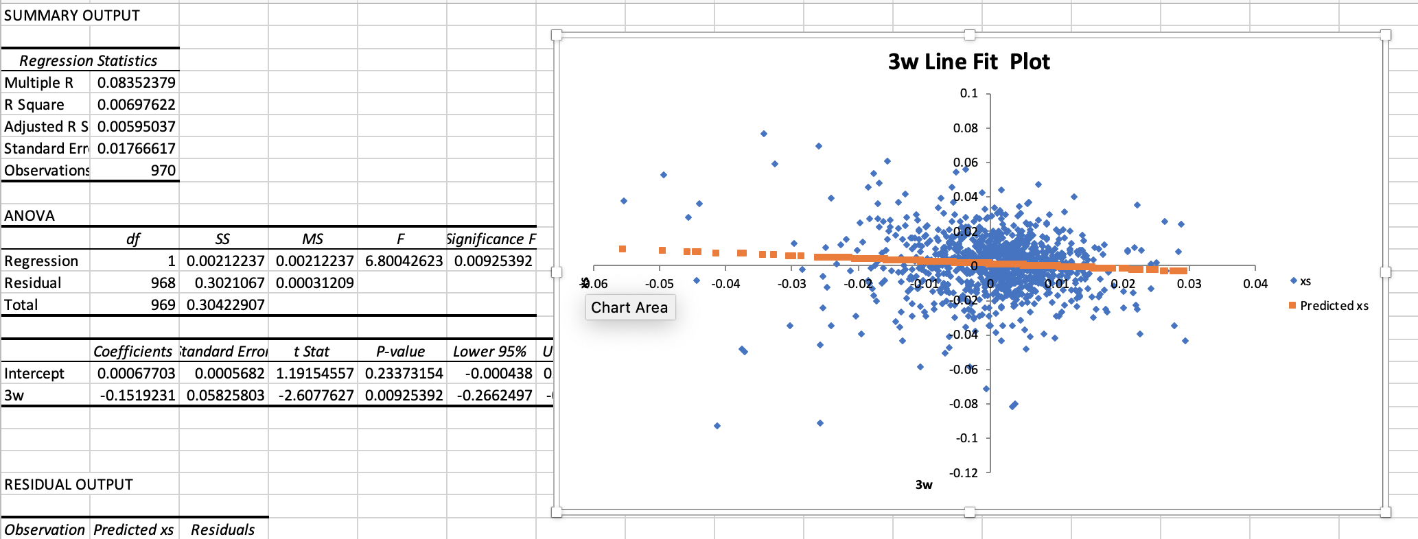
I took the weekly mean (of TLT and SPY) and calculated the excess returns of SPY for each week. I then did a simple regression of the excess 3 week returns, as the x-axis, and the following week of excess returns for the y-axis. Image below.
One of the things that is interesting is that I have real trouble acting on something like this. We do not know the closing price until the close. And we cannot act on the close until the next open (or perhaps the after-hours market).
I did not look at this data specifically but generally this type of data looks much less impressive (maybe not even significant) if you look at the next open.
I am not sure that some institutions with fiberoptic connections next to the exchanges and access to supercomputers (not to mention a lot of information on the order-flow) are as limited as I am however. Maybe they use options. Maybe they go long one asset while shorting the other (or the option equivalent). I can say that it is my experience that a lot of this gets arbitraged away by Monday morning.
One piece of data suggesting that someone may be making the market more efficient for us. I have not done the math but there is a lot that would go into arbitraging this away by Monday morning, I think. There is a lot of volume in those ETFs and the underlying assets…
Maybe I am missing something. But on first blush the regression seems impressive. And agreed. At the end of the day probably not usable. If it is usable, be my guest.
CODE:
import os
from datetime import datetime
import pandas_datareader.data as web
tlt = web.DataReader(“TLT”, “av-weekly”, start=datetime(2002, 8, 9),end=datetime(2021, 4, 1),api_key=(‘My key’))
tlt_weekly_return=tlt[‘close’].pct_change()
tlt_weekly_return.dropna(inplace=True)
tlt_weekly_return
spy = web.DataReader(“SPY”, “av-weekly”, start=datetime(2002, 8, 9),end=datetime(2021, 4, 1),api_key=(‘My key’))
spy_weekly_return=spy[‘close’].pct_change()
spy_weekly_return.dropna(inplace=True)
spy_weekly_return
cat1=pd.concat([tlt_weekly_return, spy_weekly_return],axis=1)
cat1.columns=[‘TLT’,‘SPY’]
cat1
cat1.to_csv(‘~/Desktop/cat1.csv’)