Revisiting EQUITY RISK PREMIUM

This thread continues a side-discussion from a thought-provoking thread started by Georg Vrba on June 21, 2019: "What happened to Shiller CAPE #SPPE10 "

In examining the CAPE-10 back to 1871 on the Multpl.com site, it’s clear that prior to 1990 the median PE10 was about 15, while after 1990, the median PE10 is closer to about 25. Overall valuation levels have increased by 60 to 70% in the last 30 years!

Within that thread, I asked the P123 community for ideas on why this has occurred. Specifically; “Has there been a fundamental change that increased the valuation of corporate stocks in the last 29 years?”

David (primus) answered that “Yes there has” and he provided some excellent points to consider – including:

REDUCTION OF THE ‘FUDGE FACTOR’

I can appreciate that the implication of David’s first two points would be to reduce a corporation’s ability to ‘fudge’ their earnings numbers and that valuations prior to the current era (before 1990) may – MAY – have been closer to what we are seeing today if companies were forced to provide more accurate earnings reports as a result of Cash Flow Accounting and Mark-to-Market Accounting rules. In other words, a company valued with a PE of 25 today may have been valued at a PE of 15 in yesteryear because investors took into consideration that there was a good chance those earnings were inflated. Stated differently, “Investors today have more confidence in corporate earnings and are willing to pay more.” Not sure about that, but maybe…

CONSTRUCTING AN ‘ALTERNATIVE EQUITY RISK PREMIUM’

In this post, I want to focus on David’s third comment about a more accurate workaround for the Equity Risk Premium. He proposed a formula that first inverts the CAPE-10, then subtracts out the 10-year Treasury or Corp Bond Yield to produce a “TRUE cyclically adjusted equity risk premium.”

Compared to the Fed Model, this approach has innate appeal because it would be 1) cyclically adjusted and would consider both 2) interest rates and 3) inflation (incorporated in the CAPE-10 ratio) for an Alternative Equity Risk Premium measure.

While valuation is generally accepted to be a poor approach to determining market exposure/timing, this Alternative Risk Premium might help an investor determine whether the current investment environment is ‘hot’ or ‘cold’ for equities, then perhaps other measures designed for that environment can be employed for more accurate timing decisions. Perhaps.

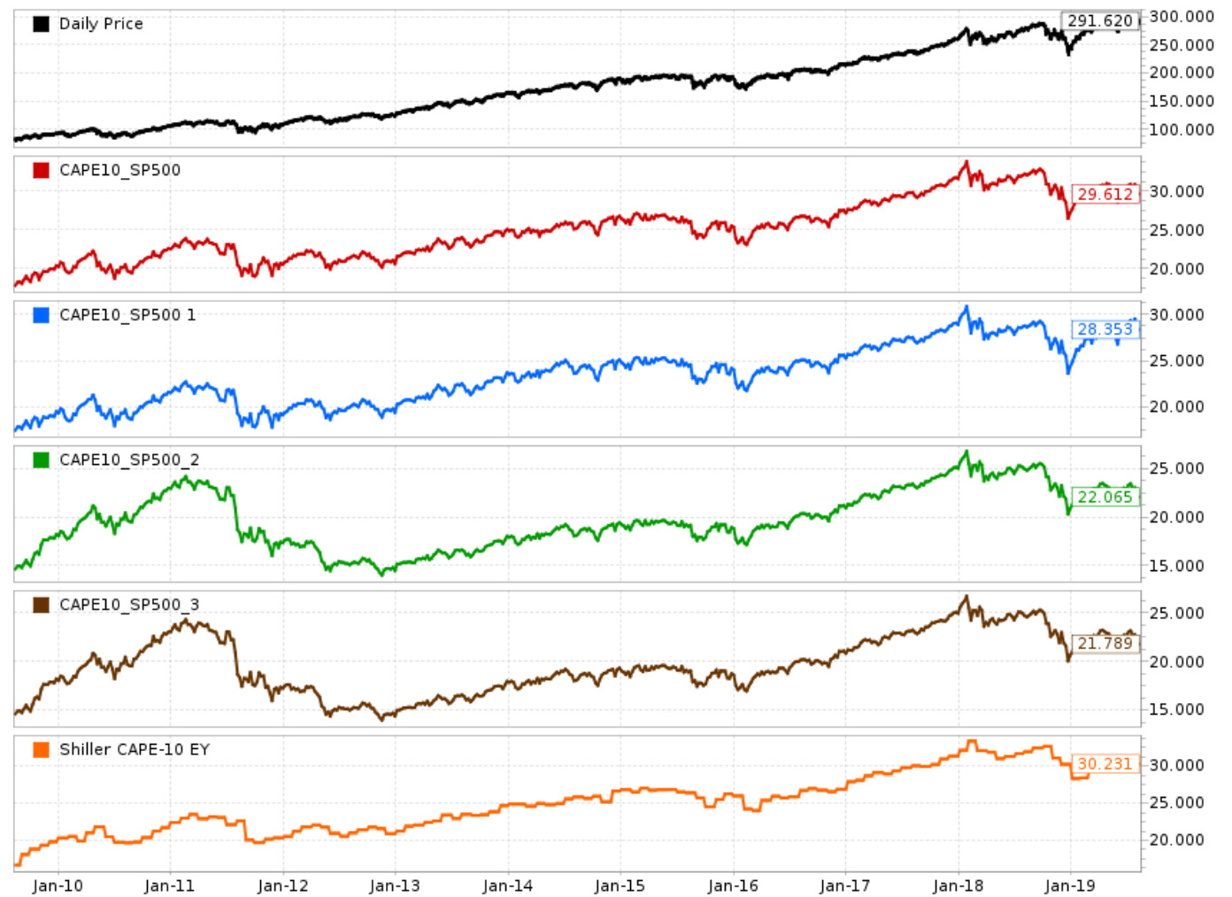
However, when creating this series, I did not arrive at “a relatively stationary time series” as David imagined. Here are the charts for the two alternatives suggested, one subtracting the Corporate AAA Bond Yield and the other subtracting the US Treasury 10-yr Yield from the inverted CAPE-10:

Alternative Equity Risk Premium (w/CorpAAA Bond Yield)

Formula: (1/(Close(0,#SPPE10)))-(Close(0,##CORPAAA))

Alternative Equity Risk Premium (w/US 10-YR Treasury Yield Bond Yield)

Formula: (1/(Close(0,#SPPE10)))-(Close(0,##UST10YR))

As you can see, it appears that these series would be less than useful for the purpose of determining the valuation or risk environment.

David, can you (or any P123 member, for that matter) address this – and let me know if I have configured it incorrectly? Thanks.

Chris

I’m not really addressing the specific question here, but here’s how I calculate the equity risk premium:

ERP = D*(1 + G) / P + G – Rf, where D is levered free cash flow (unlevered free cash flow minus interest expense plus debt increase), G is the terminal growth rate (the average of the projected inflation rate and long-term GDP growth), P is the market value of equity, and Rf is the risk-free rate (ten-year treasury bonds). So by looking at the sum of all companies’ levered free cash flow and the total value of the market, one can arrive at a reasonable premium (by my calculation, it’s 7.22%).

What if you treat CAPE-10 as the equity premium?

David, Yes; that was my understanding of the intention, but the result based on the formula you described is always a negative number (as shown by my charts). Again, here’s my interpretation of your formula:

Here’s my formula from your hypothesis: (1/(Close(0,#SPPE10)))-(Close(0,##UST10YR))

As of Aug. 11, 2019, This would be 1/29.53 = 0.0338 - 1.74 = -1.7062 (Again, a negative number, which I suspect will always be generated from this formula.)

Where have I gone wrong? Thanks

Chris

1/29.53 = 0.0338 is a ratio which has to be expressed in Pct = 3.38%
Then 3.38% - 1.74% = 1.64%

CAPE stands for Cyclically Adjusted Price to Earnings Ratio. The inverse of the CAPE would be Earnings divided by Price (E/P), currently 3.38%. As the CAPE gets smaller E/P will get bigger.

So the formula should be:
(1/(Close(0,#SPPE10)))*100 - (Close(0,##UST10YR))

Actually the Cyclically Adjusted Risk Premium is quite a good market timer.
See attached.
15 Trades - all winners, CAGR= 11.85%, and max D/D is about 30%.
Even from 1/1/2009 it outperforms buy-and-hold SPY.


Bear in mind, here, is that the equity risk premium. although a critical theoretical construct, is something that defies precise measurement because it’s an ex ante thing. In other words, we can look back and observe that the market may, over a period of time, have delivered a minus 5% risk premium, we would have to recognize the difference between ex ante, what investors expect ahead of time, and ex post, what investors actually wound up getting. Risk premium is an expectation, so when carried into the real world, sometimes the expectation is met or exceeded and sometimes life just-plain sucks.

Given the nature of what we’re dealing with, the best way to “measure” it would probably be something along the lines of how a sports media personality described the old incomprehensible and horribly confusing controversial NFL catch rule: If 20 guys watching the game on a TV in a bar think the receiver cleanly caught the ball, then its a catch. In finance, the 20-guys in a bar notion translates to an unspoken gentleman’s agreement that its about 4%-5%.

But is you want to math up here, it’s probably best to keep Occam’s Razor in mind (which should push you toward the simplest solution).

ERP = D*(1 + G) / P + G – Rf is needlessly complex because it relies on the cluster-fu** infinite growth rate assumption, twice no less, used by nobody outside the classroom to offset deficiencies in the dividend-yield start point. And the current number that comes out of it, 7.22%, would not likely be accepted by any of the hypothetical 20 guys in the bar until about 3:55 AM, when they’re completely sh**-faced and the bartender and manager are trying to shove them into Ubers over the objections of drivers who expect them to puke in their cars.

(1/(Close(0,#SPPE10)))*100 - (Close(0,##UST10YR)) is, when translated from p123 into plain English but illogical. CAPE is an inflation adjusted number. UST 10YR is not. CAPE is also a backward looking number. Risk premium is a forward looking concept. And as with 7.22%, the guys in the bar need to be ready to puke in the back seats of their 4AM Ubers in order to think 1.64% makes sense.

But at least the latter formula has some potential, assuming we correct the logical problems. If we turn CAPE around so its forward looking and and remove the inflation adjustment to make it consistent with UST 10YR, we might wind up doing this.

UST 10YR = 1.74%
SP500 Median Proj PE CY = 17.68 which flips over to an egs yld of 5.66%
SP500 Median Proj PE NY = 15.88 which flips over to an egs yld of 6.23%

That means our alternative ERPs would come in at

5.66% - 1.74% = 3.92%
6.23% - 1.74% = 4.49%

How 'bout that!

Not only would the 20 guys in a bar accept this even when they first arrive at 9 PM, if you use the Proj PE NY version and come in at 4.66%, close to the middle of their 4%-5% range, they might even pay for your drinks. And Occam won’t turn over in his grave.

One final “smell test,” (the most important test of all): Does this idea of the ERP being consistent with general ideas long held mesh with the observations of many that the stock market valuations are now very stretched. Actually, it does . . . perfectly. If you dig into macro valuations you’ll find that the main reason for the high valuation is the prolonged multi-decade collapse in interest rates which drove Rf to extremely low levels. Given that Rf is and remains within hailing distance of zero (I’m still waiting for a request I made a while back to a negative interest rate advocate to contact me off-line with a bid as to the annual rate he’ll pay me to refinance my mortgage), there are significant concerns that Rf has pretty much bottomed and will rise. That’s the problem. ERP isn’t likely to leave its current 20-guys-in-bar range unless or until there’s a major structural change in the equity market relative to other asset classes. It’s the Rf component that leads to the valuation concerns.

P.S. While I use the UST 10Y as a proxy for Rf, as do those who posted here, bear in mind this is not universally accepted. There are many who believe the term should not represent a theoretical investment horizon but be one that eliminates secondary market risk as well (i.e. the possibility the investor who needs to sell before the end of the 10th year might incur a loss in the secondary market) and per Rf at the rate of the shortest-possible term of a treasury instrument. If the 20 guys in the bar want to debate that, I choose to just find another bar in which to drink in peace.

Thanks Georg - i have never build ETF models. How does one go about doing this. Put in an Eval condition, and then if true buy SPY? What is the syntax?

Ahhh, if we only lived in Denmark. Reportedly Denmark is offering negative mortgage rates(-0.5%): https://www.marketwatch.com/story/a-danish-bank-is-offering-mortgages-with-negative-interest-rates-why-you-shouldnt-wish-for-that-to-happen-in-the-us-2019-08-12

Marc, this is only meant tongue-in-cheek. I get your unassailable logic. Still, the article is real—let me call it a one-off example of our not-so-rational market (or maybe someone has an informed reason).

Good post.

-Jim

That is correct.

There’s also an argument that ERP is the expected future earnings yield less the cyclically adjusted earnings yield.

This will also blow your minds as a market timer.

The formula is perfectly logical. The CAPE is referenced to the current CPI, so all historic earnings and S&P prices are expressed in today’s dollars. Therefore the inverse of the CAPE, which is the Earnings/Price also all in today’s dollars, can be directly compared with the current 10-year Bond yield.

Buy Rule: Eval(LoopAvg(“1/(Close(0,#SPPE10))*100-Close(CTR,##UST10YR)”,21)>1.75,ticker(“SPY”),ticker(“IEF”))
Sell Rule: 1

Note, the buy rule uses a 21-day (1 month) average of UST10YR, because UST10YR is a daily series and SPPE10 is monthly. So the model buys SPY when the Cyclically Adjusted Risk Premium is greater than 1.75%. Rebalancing is weekly.

Attached performance over last 10 years. Even during this bull market period it out-performs by-and-hold SPY.


Thanks Georg - because of your help I could create a screen

But, i could not create a sim. As i create a ranking system with no nodes, it does not allow me to proceed further. Anyone - Any ideas how to proceed?

Screen is attached here https://www.portfolio123.com/app/screen/summary/230805?st=0&mt=9

And just for full disclosure, I have multiple ways calculate cyclically adjusted earnings and P/E. While Shiller’s way is both good and canonical, there are other good approaches for achieving the same end-state.

And, oh, by the way, equity valuations do not look absurdly high now when seen through the lenses of alternative methodologies.

  • The canonical method is to use a time series of the SP500’s earnings. This will give you the CAPE for the quasi-actively managed index.
  • The alternative method is to use time-series of the SP500’s constituents’ earnings. This will give you CAPE for the index as it is currently constituted.

Which method is better?

Welcome to the multi-verse.


It does not matter what ranking system you use, because you only have one position at any time, SPY or IEF. So specify any P123 ETF ranking system and the sim will work.

Just start a New Simulated ETF strategy. Universe all ETFs.
Then put int the buy rule, and 1 as a sell rule and it will work.

Thanks Georg - but i seem to get different results. I was matching the sim with the screen. I think it is the sell rule. Does’nt 1 means sell everything? My turnover is off the charts :confused:

https://www.portfolio123.com/port_summary.jsp?portid=1580606

Regards!

Eliminate this sell rule: Rank < 80 // Sell low-ranking ETFs

Actually that rule is off

Under Rebalance:
Allow Immediate Buyback must be “yes”, you have it at “no” which results in a trade every week.

Thanks, that was it. I should have thought of that. But i really appreciate all your help.