One of the basic components of the perpetual growth model is that the terminal value of an investment is calculated by dividing the last free cash flow entry by (r - g), where r is the weighted average cost of capital and g is the terminal growth rate. The weighted average cost of capital depends on the firm’s cost of equity and cost of debt. The cost of debt is normally calculated as the average of the BBB corporate bond rate and the 30-year mortgage rate times 1 - tax rate, which currently comes out to about 2.3%. The terminal growth rate is normally calculated as the average of CPI growth and GDP growth, which over the past twenty years averages 3.16%. Now g cannot be greater than r, and if it’s very close, you end up multiplying the final free cash flow entry by a huge sum. Basically, we’re in a situation where debt is so incredibly cheap and growth is so high that the entire model seems to break down. I guess it’s what’s referred to as “negative interest rates.” Does this invalidate the model or am I doing something wrong?
Both. You’re doing something wrong because the model is invalidated under those parameters. The integral / summation for a perpetual annuity (“perpetuity) converges only when r > g.
You’ll have to break up the perpetuity into multiple annuities if you want to have g > r.
OK, the cost of debt is actually closer to 3%, and g is 3.16%. So the only way the $wacc can be less than g is if the company’s capital is about 90% from debt. And one could say that in that case the cost of equity should be enormous to make up for the increased risk of all that debt. So g would never be greater than r.
Still, though, when r is that close to g, the denominator that goes under the final free cash flow number is usually less than 2.5% and often approaches 0.5%, which means that you end up multiplying it by anywhere between 40 and 200. That just seems absurd.
Basically, when the cost of debt is lower than GDP and CPI growth, you end up with absurdly high valuations. Everything I’ve read says that I’m getting the right numbers for g and cost of debt. But maybe there’s a solution to this that I haven’t yet come across.
Maybe it’s impossible to keep this up forever
I think y’all are waxing philosophic on me. Negative real interest rates are a thing, and they imply forward growth will lag. Most schools of economics anticipate that manipulating interest rates to the downside borrows from future growth to add to the present. This is canon whether you are a die-hard Keynesian, die-hard Austrian, or somewhere in the middle. In any case, non-constant growth needs to be a consideration in y’alls mental models because high near-term growth rates don’t imply they’ll stay high.
In other words, just because g > r right now, doesn’t mean it will be like that forever. The rate of growth can exceed the discount rate for even very long periods, but growths rates are not constant. However, most simple implementations of NPV treat growth as a constant.
To capture the “stochasticity” element of interest rates and growth, we can treat future cash flow scenarios discretely, use more sophisticated models, or make some some simplifying modeling assumptions. Hey, why not do all three?
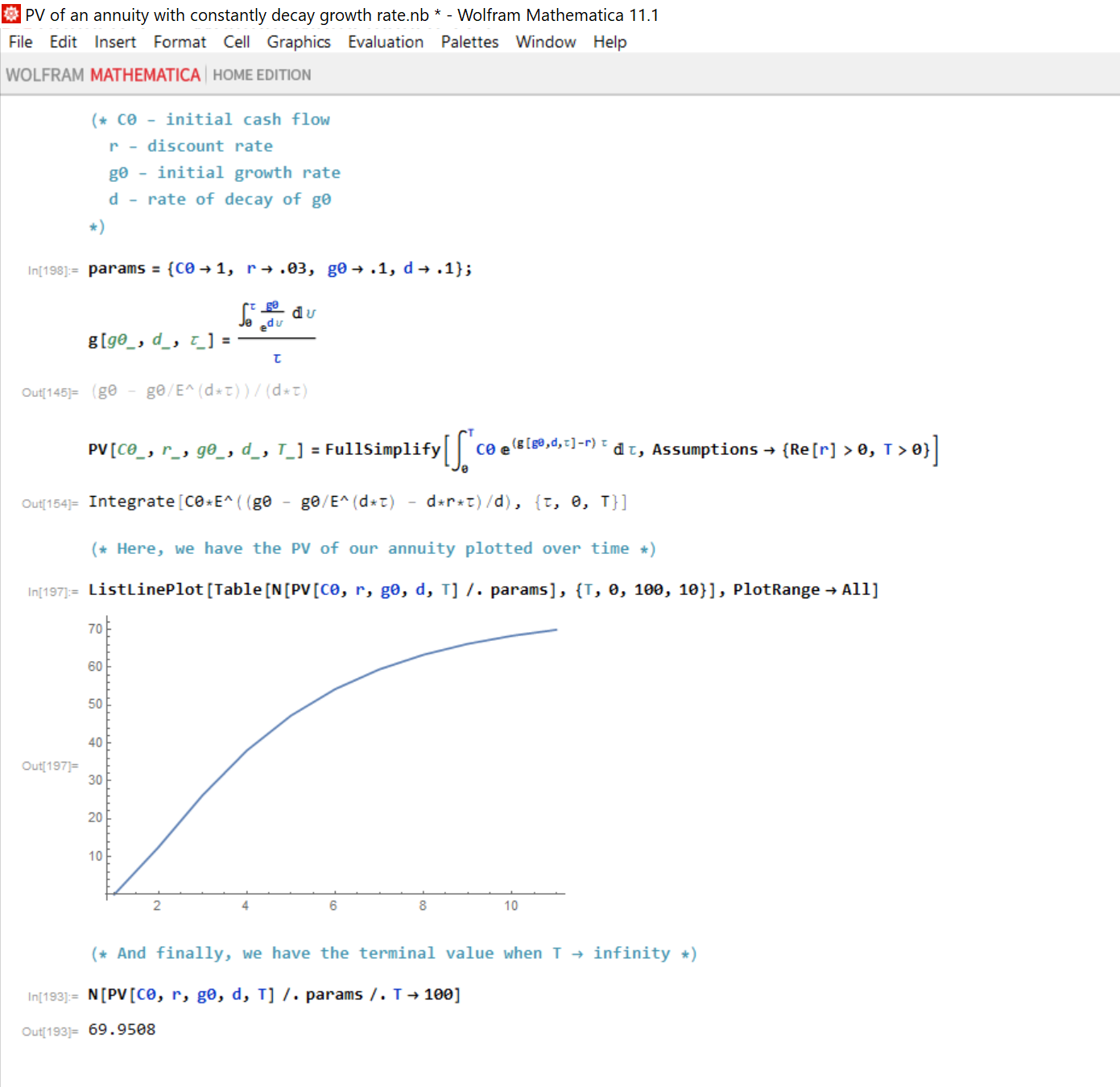
I am attaching the Mathematica code for a deterministic (i.e., non-stochastic) NPV model which allows the initial growth to decay at a constant rate. In this model, if positive initial growth decays at a fixed rate, the NPV of a positive and smooth cash flow function will always converge to a positive value–regardless of how high the initial growth rate is in relation to the interest rate.
-
Note, this model does not have a closed form solution. However, it is fairly easy to convert to a discrete form, and evaluate using LoopSum() in P123.
-
ALSO NOTE, PLEASE IGNORE THE FIRST GRAPHIC. THERE’S AN ERROR.
(* C0 - initial cash flow
r - discount rate
g0 - initial growth rate
d - rate of decay of g0
*)

In[198]:= params = {C0 -> 1, r -> .03, g0 -> .1, d -> .1};

In[145]:=
g[g0_, d_, \[Tau]_] =
 Integrate[g0/E^(d*\[Upsilon]), {\[Upsilon], 0, \[Tau]}]/\[Tau]

Out[145]= (g0 - g0/E^(d*\[Tau]))/(d*\[Tau])

PV[C0_, r_, g0_, d_, T_] =
 FullSimplify[
  Integrate[C0*E^((g[g0, d, \[Tau]] - r)*\[Tau]), {\[Tau], 0, T}],
  Assumptions -> {Re[r] > 0, T > 0}]

Out[154]= Integrate[
 C0*E^((g0 - g0/E^(d*\[Tau]) - d*r*\[Tau])/d), {\[Tau], 0, T}]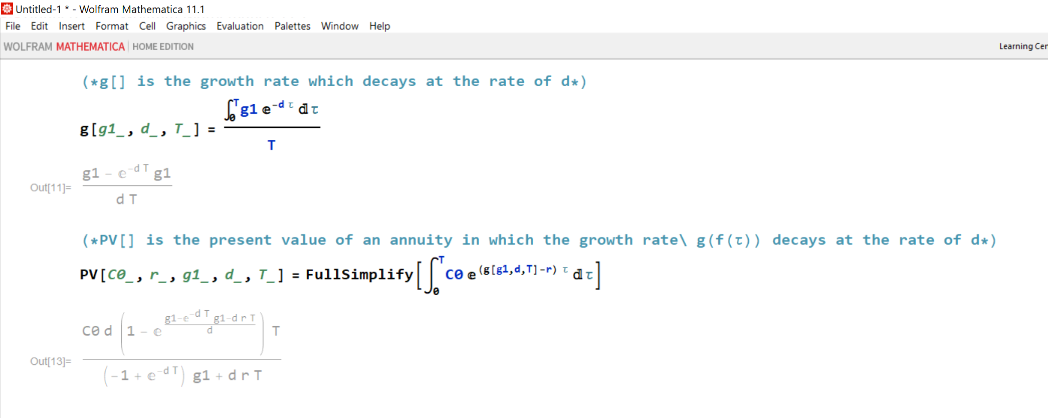
David, this is very cool! I really appreciate you taking the time and I think you’re very right about having to deal with the fact that sometimes g > r for short periods of time.
I came across a different solution, and that is to solve for g by using the equation g = (termval * wacc - finalfcff) / (termval + finalfcff), where termval is calculated using the EV/EBITDA multiples method. The median value of g over a large group of stocks according to this formula turned out to be -0.61%.
But there’s considerable appeal to a constantly decaying g. I may try to use it.
The other thing I found interesting when thinking about all this is that nobody talks about the period, which is the hidden variable in the formula P = D/(r-g). If you look at Gordon’s growth model, it’s really elegant in its mathematical simplicity. But if you change the period, P changes quite drastically.
Let’s say you have three stocks. One starts out paying a $120 dividend once a year. One starts out paying a $10 dividend once a month. And the third starts out paying a $600 dividend once every five years. The total payments into perpetuity are exactly the same. All of them have an annualized growth rate of 5% and all of them have a required return of 10% per year.
The value of the first stock is $120 / (0.1 – 0.05), or $2400.
The value of the second stock is $10 / (1.1^(1/12) – 1.05^(1/12)), or $2,564.09.
The value of the third stock is $600 / (1.1^5 – 1.05^5), or $1,795.18.
In other words, the price is dependent not only on the amount of dividend, the rate of growth, and the required return, but also on the period of payments.
I don’t know if it’s appropriate to apply this to the NPV formula, which should probably be based on quarterly rather than annual periods, but it’s an interesting twist.
First, as to the negative interest rates . . . somebody here said its a real thing. OK. I’m convinced. I’m in. Please contact me off line. I want to refinance my mortgage, and we’ll talk about how much you’re going to pay me for the privilege of making the loan.
Second, yes, you are absolutely positively doing the wrong thing. Horrifyingly and comically wrong.
The (r - g) thing is theory. It’s not a formula into which you can plug numbers. Please read this article. Although it critiques “physics envy” in terms of social science research, it applies equally well to investing:
The whole article is important, but here’s a quick summary of the salient point: “To borrow a metaphor from the philosopher of science Ronald Giere, theories are like maps: the test of a map lies not in arbitrarily checking random points but in whether people find it useful to get somewhere.”
That’s what the Dividend Discount Model is. It’s a map that can be useful in helping investors get somewhere (from a mish-mash of ideas to a viable strategy).
I have a friend who assesses hotels for a living. I asked him if he uses the discounted cash flow model to do so. He said, “Yes, that’s my number-one model.” Michael Mauboussin, a writer and investor whom I really respect, has written a book on the DCF model (Expectations Investing). I also know that all financial analysts have to understand the DCF model and pass tests on it. So it seemed worthwhile to learn it myself.
And an important component of the DCF model is dividing terminal value by (r - g), where r is the WACC and g is the terminal growth rate. That’s the hardest part of the model for me to understand, which is why I started this post.
Yuval,
Everyone who has posted so far knows WAY more about this than I do.
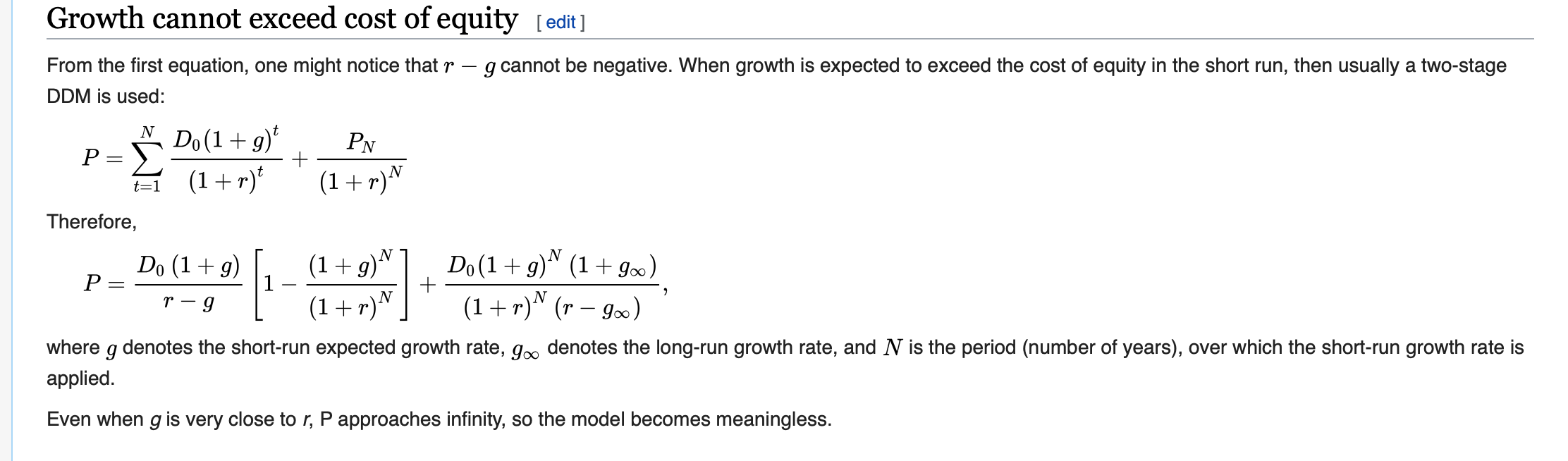
I do not know if this helps so I attach the image from Wikipedia (DDM) without comment.
-Jim
My humble recommendation is to understand series summations, Reimann sums/integrals, and Volterra integrals. Once you have that down, play with these in Mathematica.
PUBLIC SERVICE ANNOUNCEMENT FOR MAINSTREAM P123 USERS:
If any of you are intimidated by what you see in this thread, rest assured that absolutely NOTHING being discussed is of any relevance to real-world investing.
If math fans want to discuss what they want to discuss, that’s fine. But over the years, I have heard feedback about members feeling intimidated when they see discussions like this, and fearing that p123 may not be for them.
Rest assured that if you are not into this sort of thing, you lose nothing. If you like this sort of thing, join in. Otherwise, feel free to ignore everything here.
END OF PUBLIC SERVICE ANNOUNCEMENT
That being said, have at it guys.
Marc,
LOL!!! For the record I have tried to plug some P123 factors/ratios—more or less trying to duplicate the DDM—into a ranking system. Seems someone recommended this to me. Nothing as mathematical as above, however.
Maybe not wanting to divide by zero (even in a ranking system) is advanced—so maybe a matter of interpretation. I did not mind the explanation (in the reference) that perhaps the situation (of a zero, near zero or negative denominator) is temporary. Of course, I am not claiming that this describes the present situation. This is your area of expertise and it is a formula you have used (and recommended) a lot.
In non-mathematical terms what is the present situation and what does it say about what we should do?
-Jim
So if this conversation is of no relevance to investing whatsoever then, by logical association, r-g must also be irrelevant because it is directly derived from a summation (or integral) of the discounted cash flow formula. I have no issues with your egalitarian attitude, but I feel like if someone doesn’t have a grasp of the fundamentals of time value, then we are within scope to revisit the basic financial theory.
(* Formula for simple growing annuity using Riemann integral *)

In[114]:=
PV[C0_, r_, g0_, d_, T_] =
 FullSimplify[Integrate[C0*E^((g - r)*\[Tau]), {\[Tau], 0, T}],
     Assumptions -> {Re[r] > 0, T > 0}]

Out[114]= (C0 (-1 + E^((g - r) T)))/(g - r)

(* Formula for simple growing perpetuity using Riemann integral \
(note, PV[] is only defined for g < r *)

In[148]:=
PV[C0_, r_, g0_, d_, T_] =
 FullSimplify[Integrate[C0*E^((g - r)*\[Tau]), {\[Tau], 0, Infinity}],
     Assumptions -> {Re[r] > 0, T > 0}]

Out[148]= ConditionalExpression[C0/(-g + r), Re[g] < Re[r]]

(* Formula for simple growing annuity using Riemann sum *)
(* Note that this provides a solution for Fischer's real interest \
rate equation: https://en.wikipedia.org/wiki/Fisher_equation *)

In[180]:=
PV[C0_, r_, g0_, d_, T_] =
 FullSimplify[
  Sum[(C0*(1 + g)^(\[Tau] - 1))/(1 + r)^\[Tau], {\[Tau], 1, T}],
     Assumptions -> {Re[r] > 0, T > 0, g < r}]

Out[180]= (C0 (-1 + ((1 + g)/(1 + r))^T))/(g - r)

(* Formula for simple growing perpetuity using Riemann sum (note, \
PV[] is only defined for g < r *)

In[181]:=
PV[C0_, r_, g0_, d_, T_] =
 FullSimplify[
  Sum[(C0*(1 + g)^(\[Tau] - 1))/(1 + r)^\[Tau], {\[Tau], 1,
    Infinity}],
     Assumptions -> {Re[r] > 0, T > 0}]

Out[181]= C0/(-g + r)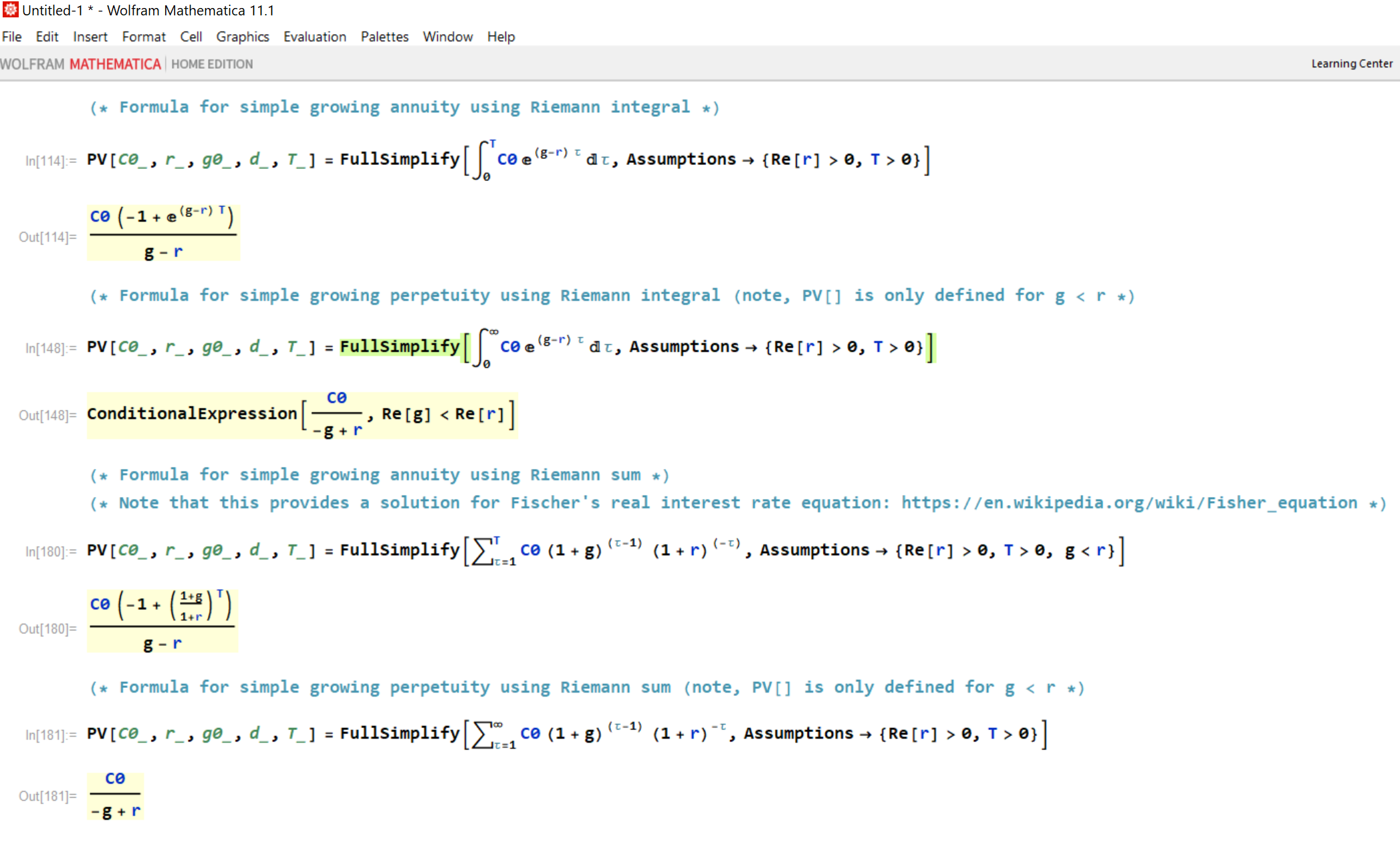
For those who insist on trying to make a mathematical thing out of (r - g), please read the quote I used in a prior post from the physics envy article regarding the role of theory, as well as the article itself . . . And by all means please go back to the material in which I initially presented the model, in which I made it clear that it is NOT a formula into which we can or should even try to plug numbers.
Marc,
So the question is just how “fuzzy” the information is. Is it concrete and specific enough to be actionable?
What, in non-mathematical terms, is it telling us to do now? You have made predictions about what kinds of stocks will do well based on this in the past. Will that work now?
I get your point. For sure, I am not about to do any integral calculus myself. But you have said it is an important formula. Tell us–in your own terms–what the DDM is saying now.
Which is more true about long-term investing?
-
The DDM has some ability to determine which stocks to invest in, or
-
“Want to know what’s going to happen in the next year? No problem; I’ll tell you 366 days from now.”
-Jim
Interesting discussion. If one does not use some form of DCF (multiples being the shorthand), how does one value a company?
I’m writing an article on that. It’s over 4,000 words long at this point. It should be finished in about ten years (just kidding).
For what it’s worth, Graham and Dodd wrote in Security Analysis:
We must recognize . . . that intrinsic value is an elusive concept. In general terms it is understood to be that value which is justified by the facts, e.g., the assets, earnings, dividends, definite prospects, as distinct, let us say, from market quotations established by artificial manipulation or distorted by psychological excesses. But it is a great mistake to imagine that intrinsic value is as definite and as determinable as is the market price. . . .
[The] concept of intrinsic value, as . . . definite and ascertainable, cannot be safely accepted as a general premise of security analysis. . . .
The essential point is that security analysis does not seek to determine exactly what is the intrinsic value of a given security. It needs only to establish either that the value is adequate—e.g., to protect a bond or to justify a stock purchase—or else that the value is considerably higher or considerably lower than the market price. . . .
To express the uncertainty of the picture, we might say that it was difficult to determine in 1933 whether the intrinsic value of Case common was nearer $30 or $130. Yet if the stock had been selling at as low as $10, the analyst would undoubtedly have been justified in declaring that it was worth more than the market price. . . .
It would follow that even a very indefinite idea of the intrinsic value may still justify a conclusion if the current price falls far outside either the maximum or minimum appraisal.
And I came up with a reasonable solution to the problem I started this post with. The cost of debt for most industries should not be measured by the rate of BBB bonds (or the thirty-year mortgage rate) but by the rate of B bonds, which is significantly higher. There are exceptions–utilities, for instance, have a very low cost of debt, and the cost of debt for staples is pretty low too. But on the whole, this, together with a higher-than-I’d-thought equity risk premium, solves the problem.
As to Marc Gerstein’s point, I agree with him 100% that actually doing DCF analysis is by no means necessary to be a good investor. It could actually make you a worse investor! But I think UNDERSTANDING it may be important. It gives you a real perspective on how money is SUPPOSED to work. P = D / (r - g) remains a very abstract concept until you actually start plugging in the numbers and seeing how it works (or doesn’t).
Moreover, for math nerds like me, it’s kind of fun.
My understanding is that DCF is only useful in application to companies that have an economic moat, and even then one has to establish a bear case (minimum growth). Morningstar has been doing this for several years, have 100 analysts working on this and the result is the ETF MOAT which does perform slightly better than the S&P 500. This is with many analysts doing manual analysis, not pushing a button to tap a database, using the most predictable stocks (economic moat) to determine fair value.
So yes, DCF does work to some extent but is probably not practical on this platform. For most stocks, it is really a case of choosing what assumptions you want to use and running with it.
I also believe that you guys are getting carried away with applying theoretical mathematics to the markets. The markets will beat you at this game.
Marc has used what is really the Gordon Growth Model, I think, which replaces r with k
where “k” represents the “required return rate for the equity investor.”
He relates “k” in different environments to risk, the expected direction of interest rates etc.
Whether it actually works or not, it gives me reason to think there may be some rational explanation for why my stocks seem to be influenced by the FED’s decisions.
Anyway I am a big fan of the idea for predicting risk on/off, interest change affects on stocks etc. I cannot verify that it could work for me if I tried to make any predictions. But I suspect it could be useful in Marc’s hands. I have no series or track-record of predictions to look at with regard to the accuracy of predictions. I hope no one thinks my questions were intended to put anyone on the spot.
-Jim