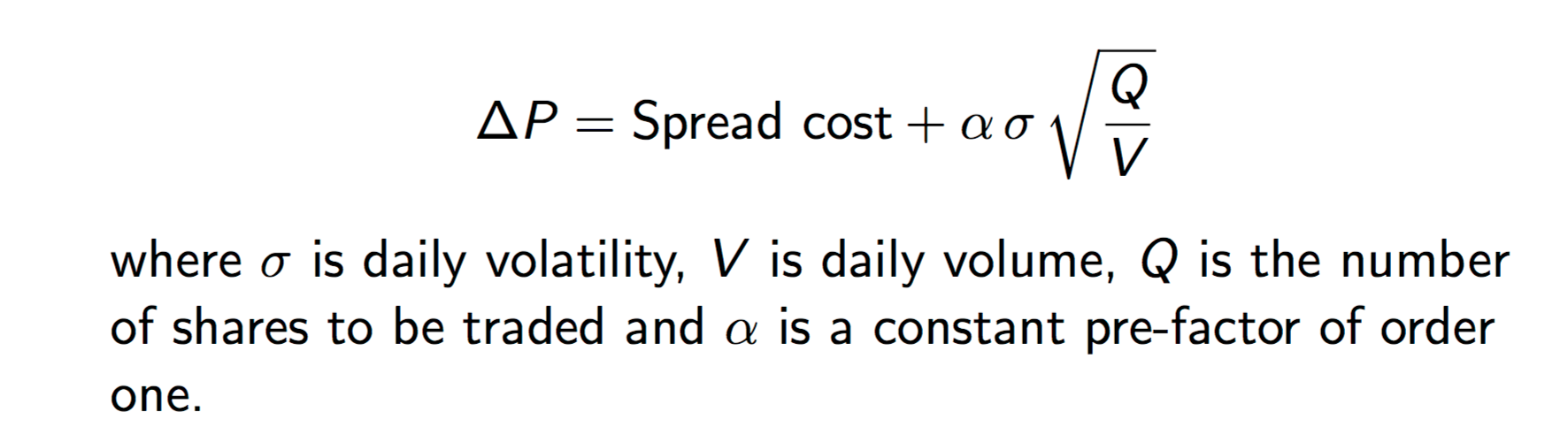
Multiple sources show that the equation for slippage includes the term (Q/V)^0.5. Where Q equals the quantity of stocks purchased and V equals the total volume of stocks traded that day.
But this is the cost of the nth stock I buy.
To get the total slippage for all of the stocks that I purchased I would have to integrate that wouldn’t I? I want to know the area under the curve for the costs of each stock. If I buy 5,000 stocks the last stock will cost more than the first and I want to know the cost of all of the stocks I purched: not just the last stock I purchased.
So if that is the case then my total costs equation should include the term (Q/V)^3/2, I think. By integration.
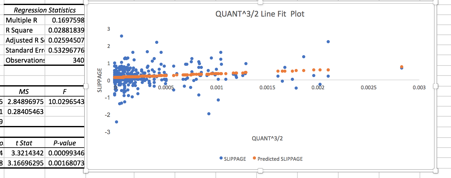
In a linear regression for stocks I have purchased this year using window trades this seems to provide the best fit. See attachments.
I find this useful for determining questions such as: What will happen if I double the amount of money in one of my ports? What is the maximum liquidity this port will allow?
Using “predict” in R, I seem to be getting pretty accurate answers to these questions—so far.
And generally my estimations of slippage seem much more accurate because every purchase that I have made affects my calculations for slippage. By this I mean that a single port may have an outlier(s) that may affect the calculation of my slippage for that port. But if I know the average daily volume of the stocks traded and the average quantity of stocks I purchased for that port the calculation using the regression is a better estimate of what the slippage will be in the future.
Again “predict” in R is helpful for this but the calculations can be done with a hand calculator (or in Excel). Just remember the commutative and associative properties allow you to use averages (being a little careful about when you use the ^3/2 power).
This may or may not be useful for your type of trading. Any ideas on improvement welcome.
So let’s assume you buy 3,000 ETF VTI on 4/13/17 @ $120.00. That is a trade of $360,000, not an insignificant amount.
04/13/17: open=120.15, Hi=120.56, Lo=119.55, close=119.55, V=2,850,692
Then according to your formula expected slippage= (3000/2850692)^1.5= 0.000034= 0.0034%, basically zero slippage, as this trade is too small to affect the price.
If this is this correct, then the min slippage for ETF Designer Models should not be 0.1%.
For a slippage of 0.1% one would have to trade 28,500 shares for $3,420,000.
Thank you. If you do your own regression with your slippage data you will have a y-intercept.
The equation will be slippage = m(Q/V)^3/2 + b. So you will find your own “b” that will be above zero slippage. I did not include that part of the Excel regression because it would not be useful (probably) to your liquidity and for your trading method. You will also find your own “m” or slope of the line.
In practice would “b” end up being the BID/ASK spread or 1/2(BID/ASK) spread for stocks with very high daily volumes? I don’t know but this would seem to be the lower theoretical limit. My regression is very accurate and it doesn’t seem to matter. But I did not mean to give the impression that the y-intercept would be zero.
It is a little more math than I like but in the end it is just a linear formula and a linear regression with manipulation of (Q/V) first.
I’ve borrowed a lot from Robert’s work, but I am unconvinced regarding the presence of 3/5 power law. The null hypothesis is still that the root power law should be the one observed (Jim Gathedral’s work on the differential math contains the best proofs, I think). I think the failure to confirm the root power law is a result of: a) noise; and, b) the inability of the model to capture a key dynamic. Therefore, I still use the root power law.
I see myself as having zero edge in short-term trading, so I quantify my expected trading costs in terms of slippage + commissions + temporary impact + permanent impact. If the expected costs do not overcome the expected upside, then I trade. Philosophically, that is what I view as the proper role of trading to an investor: to quantify the expected net costs and come up with strategies for efficient execution.
On a side note, I think that all the stuff we continuously get bombarded with on CNBC, Bloomberg, and elsewhere about trends, patterns, etc is just “useful fiction”. It’s useful to sell-side analysts and brokers who benefit by increased activity; it may be useful or counterproductive to other market participants; it’s not useful to me, though. The problem with any sufficiently convincing myth is that it is both well-intended and insidious. Our brains are wired to pick out patterns which have historically resulted in increased chances of survival and reproduction. In the wild and in the human worldly experience, these patterns are more often than not useful. In the casinos, however, they are just counterproductive remnants our of primal selves.
Anyway, if anyone is interested, I can send them a copy of a screen which implements the Almgren canonical estimate of cost with intraday variance estimation using the Yhang-Zhang (YZ) OHLC estimator. YZ is the most efficient estimator out there without the use of true intraday day.
I saw this and tried incorporating volatility of the stock for a while. I am a bit lazy.
Do you get that this is the cost of the nth stock and you would integrate the equation to get your total slippage? It makes a big difference. I see the end of my liquidity–in the not too distant future–if total slippage increases by a power greater than 1.
The pattern of my residuals did not look good at all when, naively, I tried a regression with (Q/V)^1/2. So bad that I stopped recording the daily volumes for a while which is why I do not really have that many data points.
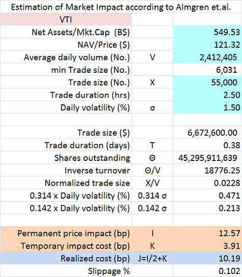
Using the Almgren formula one would get a slippage of 0.1% for a trade of 55,000 VTI ($6.7M), assuming the trade is spread over 2.5 hours.
So the P123 requirement of 0.1% slippage for ETF DM-models is very conservative.
However, doing the same calculation for VOE, one would get a slippage of 0.1% for a trade of 8,700 VOE ($0.88M).
I studied my slippage trading costs (for close to 3000 stock trades, with every stock trade including multiple transactions).
I looked for slippage in relation to opening price of the day, which is before I start to trade.
My best fit for TOTAL slippage % (not just for the last stock traded) calculated as the difference between AVERAGE trade price and opening price, turned out to be: Slippage % = 0.02*my volume % of daily traded volume^0.5.
Since I trade almost exclusively in microcaps using limit orders, the traditional equation isn’t terribly applicable to my slippage costs, which average around 0.5% or 0.6%. Here’s the reason. If I’m buying 2% of the average daily volume of one stock and 50% of the volume of another, the traditional equation says that my total slippage will be five times higher for the second buy as it was for the first. (If I were to use Jim’s formula–raising Q/V to 3/2 instead of 1/2–it would be 125 times higher, which is a real problem with Jim’s formula IMHO.) These huge differences are not at all what I’ve experienced; and the conventional Q/V formula was not meant to apply to microcaps or buys of 50% of daily volume. My slippage is roughly inversely proportional to the logarithm of the average daily dollar volume of the stock, and is not terribly affected by the volume of my buy. My formula for slippage is 0.054-0.0039*ln($vol), so a dollar volume of $20,000 gets a slippage of 1.5%, a dollar volume of $100,000 gets a slippage of 0.9%, and a dollar volume of $1 million gets a slippage of 0.01%. With dollar volumes higher than $2 million, I experience negative slippage–in other words, my limit orders get filled, on the average, at a better price than the opening. Now by not factoring market impact into my slippage costs, I may be underestimating the cost of large buys, and I might change my estimating mechanism in the future. But I doubt I’m going to be using (Q/V)^0.5. Maybe (Q/V)^0.2 . . .
No, I’m assuming that the bid/ask spread is very large for stocks with low dollar volumes and smaller for stocks with high dollar volumes. My slippage estimation is not very far from that employed by P123 in their variable slippage formula.
Just did not see the BID/ASK spread in this calculation.
I had to actually do the regression to get the Y-intercept.
BTW, if someone else gets a different power for best fit when they do a regression that means they get a different power. I’m just sharing my regression and my rational for using (Q/V)^3/2. (Q/V)^0.5 did not work for me. I tried it.
Interesting that I got a higher R (or R^2) than Almgren did. That could change as I get more data but I’m inclined to keep looking at it—for my window trades.
And actually, if anyone has done a lot of calculus recently, I would be interested if my calculation is that different from a simplified Almgren’s. I do not think my equation is much different than Almgren’s. I posted, in part, so you guys could check that. My equation is integrated and simplified, however.
I get that there can be separate constant when you integrate but wouldn’t the constant before integration be zero. The constant after integration becomes part of the Y-intercept in the linear regression. I also get that there is a constant in front of (Q/V) that need to be adjusted with integration (i.e., 1/2C(Q/V)^3/2) but if I am finding this constant when I do the linear regression there is no need to put a constant in front of the term (before or after integrating). It is found by the linear regression.
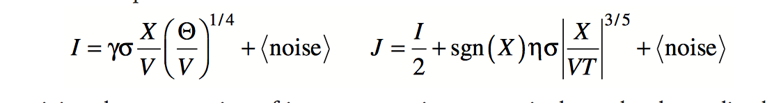
In other words won’t Almgren have a term C|X/VT|^8/5 in his equation when he integrates? And won’t he want to integrate if he wants to know the cost of each stock he buys? Unless there is a big difference between 8/5 and 3/2 I’m not sure there is a big difference.
In any case, for now, I do not think I am disagreeing much with Almgren. And there may be other formulas where I may be in complete agreement (see attachment on my original post). In agreement except that I do not include a stock volatility term. Also, any agreement (or disagreement) may depend on how you view the Y-intercept of the linear regression in relation to the BID/ASK spread. I think theory supports the idea that the Y-intercept is 1/2*BID/ASK spread of stocks with large daily treading volumes for my linear regression.
Whether I am correct about the theoretical meaning of the Y-intercept does not matter to me. For now I am please that I have a R that is good. Better than Almgren’s published data. So far the linear regression just works.
Whatever you do on this remember, Almgren is just looking at the market impact on the nth stock purchased: NOT SLIPPAGE!!!However you may want to calculate slippage that is not what Almgren’s equation is calculating. Related but not the same.
Do not use his formula alone–or the one in my first post’s image–to calculate slippage!!! Well, if you have a factor for BID/ASK spread you could be close. Could be but you should test it against your own trades. I could not get it to work for me (which resulted in the above posts).
Thank you yorma. Like I said, if you get different numbers its is because you get different numbers (just different data). Or because you don’t do window trades (probably): who knows. But it is interesting. Any discussion would be whether my integrated equation is correct. Maybe there is a constant in the integration that I did not account for (not zero as I said with a cx term missing in my equation). But if you are starting with the market impact then adding in the BID/ASK later, someone would have to explain that to me. Or whether it should be integrated (theoretically) in the first place: okay no doubt on that. You want the area under the curve. But my regression does not have to work for everyone.
And in fact, I take no responsibility for those who cannot plug in a few data points into their Excel spreadsheets and determine the power that best fits their own data. “Results not typical. Your results may vary.” “Do not try this at home.” “Please, consult with your own financial advisor.”
There are two issues here: slippage does not equal impact; and the integrated market impact of an arbitrary buy or sell order.
I agree that slippage is not the same as temporary and or permanent impact on price. But both things affect the price we pay end up paying to enter and/or exit a position, hence the conflation.
The reason why I think market impact and slippage costs get conflated is that neither can be directly observed. It would be nice if we had a time machine to ask the question “what would have Monday’s open and close price been had I not traded those days?” However, no such time machine exists. Implicit costs are fundamentally different than direct costs, i.e., commissions and taxes.
That was not my interpretation. If the author intended practitioners to integrate the cost on a share-by-share basis, why does he then use the ratio of purchase/sale shares over average daily volume? Consider the following:
If the market impact is just realized change in transaction price, wouldn’t a VWAP order just result in slippage equal to one-half of the expected price change?
Take, for example, the generic model given on page 61 of the following document: Faculty Profiles
If you integrate the inside of the integrand with respect to v, you do indeed get 3/2 power law. However, it is differentiated with respect to s. For t-s = 1 (i.e., you place a one-time order at the close), the integral is linear and defines itself as its derivative.
But then again, if you your own execution data supports the 3/2 power law, then it probably captures a unique dynamic of your execution strategy. “If ain’t broke, don’t fix it” seems apropos.
Jim,
I suggest you check the following study: “Trading Costs of Asset Pricing Anomalies” http://faculty.som.yale.edu/Tobiasmoskowitz/documents/TradingCostofAssetPricingAnomalies.pdf
My results are quite similar to those shown on figure 2 “Market Impact by Fraction of Trading Volume” (Page T13).
If I understand correctly, in that article “market impact” is defined as total transaction loss (not just the loss of the last trade).
And considering the title of the paper “Direct Estimation of Equity Market Impact,” I share your concerns—in spades.
The paper delivers, as promised, on its title when it gives us equations for " the permanent price impact" and the “temporary impact.”
I will look again to see when Almgren makes the switch to a comprehensive slippage calculation that could be used–without modification–by investors at P123. I probably just missed it. Either way, it is a good paper and I appreciate the link and the discussion of it. It is one I looked at before.
A note to those who have not looked closely at the equations: There is no factor or constant for BID/ASK spread in the final equation. He does address BID/ASK spread and its effect (or lack of effect) on “Equity Market Impact.” He does not include it because of its lack of effect for what he is looking at.
What would your total slippage be when you buy just one stock? Near zero market impact as the equations suggest. But I am guessing there would not be zero slippage for a market or window order (as in my case). Because of the BID/ASK spread. I am guessing that you might have to pay at least a nickel at times. Okay, to be honest, I have tried this for window trades to get a "control’ or a “baseline” for calculating by personal market impact. I am not guessing. I know the answer on how much percentage slippage there is for a single share: A LOT. NOT ZERO!!! Not near zero.
For me, for my trades, the BID/ASK spread (or a constant incorporating it) has to be somewhere in my equations. Especially, with the nickel spreads.
And this has changed. Perhaps, due to the nickel spreads but can you use any equation over a year old?
You may have to modify the equation for this (or other reasons) too. Start by changing nothing else if you want to—assuming the consideration of BID/ASK spread applies to your trading style. Let me know how it works. And if the 3/5 or 1/2 power does not work then think hard about what the title of the paper says. You may—or may not— be able to find a rational reason to try another power. It is not a simple formula and if you are like me you may seek to simplify it (if nothing else). But if you start there you will be starting where I started. It is taking me a while to get it: everyone, including those who think I never got anything on this, will have to agree with me on that.
David, do you have any data you can share? Did the formula work strait out of the box for you? Did you modify any of the constants based on regressions of your own data? If you have modified it, how do you address BID/ASK spreads with your microcaps? Maybe you use limit orders.
It is a good formula and I am all for people using it with any modifications that you may feel are appropriate. But strait out of the box?: not so much.
Whatever people do: If it works, it works. And that works for me.
-Jim
Thanks!!! Still early. I will definitely check that out today.
And I will keep looking at my data. If (Q/V)^1/2 (or ^8/5 for that matter) ends up working best for my data I will let everyone know.
This post also allows me to make some corrections: in my ideas. My data was correct to the best of my knowledge.
@ David (Primus) I now agree with you that ^0.5 or possibly ^3/5 is the correct power
@yorama. It was your quote that made me understand. While my integration may have been (or may not have been) correct I was not calculating the average trade price. This is what you were trying to tell me, I think. For a moment, I thought you were stressing the need for integration of the price impact.
I could spend a lot of time on why I was wrong. But I was having real troubles with this when I tried it before and adopted (Q/V)3/2—perhaps I did not have enough data points with good scatter in the right portion of the x-axis. My last check of the data—that I posted—made me think I was on the right track (confirmation bias). ^0.5 seems to be working better now.
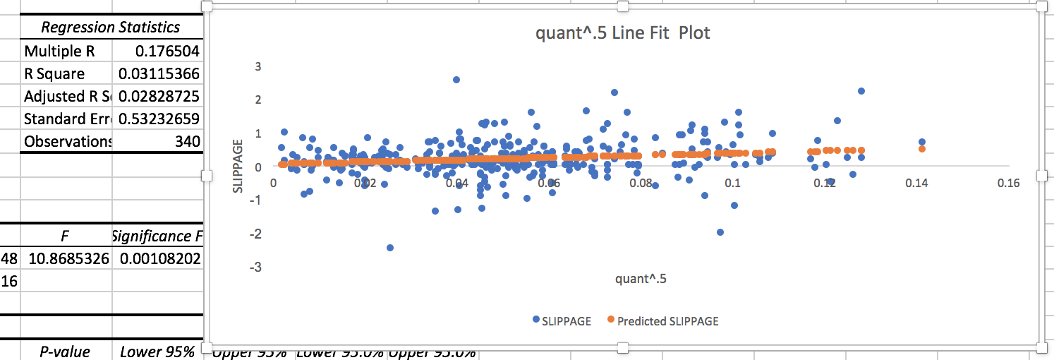
I do not think I would have tried ^0.5 again without your posts and I am almost certain that I would not have realized that ^3/2 is just wrong and has no theoretical support or basis. For those who have any interest in this topic I have redone the same data in the original post with (Q/V)^0.5 on the x-axis. As you can see scatter plot has a better appearance and the R^2 is better than the one in my original post.
Again, all of your comments are greatly appreciated and were very helpful. And I apologize for being slow to understand.
I just wish I could change the original title of this thread.