I’ve been racking my brain for a week trying to figure out a good way to create a time-series for a custom “capitalization weighted” benchmark for different markets/sectors/industries using the GICS code. The result will be used for personal research; it is not intended to be used further inside screeners/portfolios (although that would be nice). According to the info sheet on the Series Tool, we should be able to “Create your own benchmark”. The example custom benchmark given to us is a price weighted (as opposed to capitalization or equal $ weighted) basket respresenting a fixed list of stocks; it is not representative of a capitalization weighted index, like the S&P 500. Also, when using the GICS, stocks get added and removed from the index; therefore it needs to be continually readjusted to reflect that fact.
I am using guidance from S&P’s capitalization weighted methodology to attempt to construct a time-series for a benchmark of “gold miners” (GICS 15104030). My intended approach would be something very similar to how S&P constructs the S&P 500 index. Just like the S&P 500, a GICS sector/industry is not a fixed basket of securities. Therefore, simply summing the market capitalizations (or the investable portion therefore) for all stocks in the GICS won’t work because as new stocks are added or removed, this will increase or decrease the value of the index. Only capital appreciation/dividends should increase/decrease the value of the index, not additions/subtractions. To restate this, adding or removing stocks from the index should not change the value of the index.
I think I would be able to estimate the value of the index if I had access to historical information about which stocks were in the GICS. Knowing how much money flowed into and out of the GICS over some timeframe would allow me to adjust the value of the index such that additions/subtractions would not change the value of the index. However, the only way I know to get that information is through something like, FHist(“GICS(15104030)”, 1). However, I would need to access FHist through a universe function inside quotes; nested quotes are not possible in P123 so I need to find another way. Does anyone know of a way using the Series Tool to compare what the stocks in this industry are and what they were last week?
Moreover, does anyone know how to approach solving this problem inside P123?
A final note: I am not so much concerned about all the fancy things S&P does with corporate actions, investability (i.e., float adjustments), et cetera. All I want to do is come up with a way to compare performance against an investable “capitalization weighted” benchmark.
An interesting approach will probably get me 99% there. S&P’s guide on indexing methodology, Equation (2) describes a LasPeyres index. Basically, its says you can look at the price change to determine the index. That said, my implementation looks like:
UnivGICS(15104030)
setVar(@MktCap_Bgn, UnivSum(“SharesCur(0) != NA AND CloseAdj(0) != NA AND SharesCur(1) != NA AND CloseAdj(1) != NA”, “SharesCur(1)*CloseAdj(1)”))
setVar(@MktCap_End, UnivSum(“SharesCur(0) != NA AND CloseAdj(0) != NA AND SharesCur(1) != NA AND CloseAdj(1) != NA”, “SharesCur(0)*CloseAdj(0)”))
SetVar(@Rtn, LN(@MktCap_End/@MktCap_Bgn) )
The result will be the daily logarithmic change in the index. If you know the log change, you can calculate the index value by applying the natural exponent to the power of its cumulative sum of log returns… whatever all that math means.
The point is, I think this might be “good enough” solution which is capitalization weighted and is unbiased for additions and subtractions (except for a 1-day look-ahead bias, if that even matters). My questions now are:
In the above, I use CloseAdj(). Is this the right way to do it? I.e., is SharesCur() backwards adjusted for splits as well?
Can I make any additional adjustments to remove look-ahead or other bias?
I think this is an important topic because custom benchmarks was a widely requested feature. Simply put, the ability to compare your screen’s / portfolio’s performance against an appropriate “dumb money” index will let you know how much “gold” or “fool gold” might be in your methodology. Comparing an equal $-weighted basket of small-caps chosen according to some rules against the S&P 500 is ludicrous. Now, comparing your equal-$ weighted portfolio against a “dumb” index consisting of the base universe from which you applied your selection criteria is SMART. If we can all get on board with the “right” way to calculate benchmarks, I think we can all greatly profit.
Would love to hear feedback/criticism from the community.
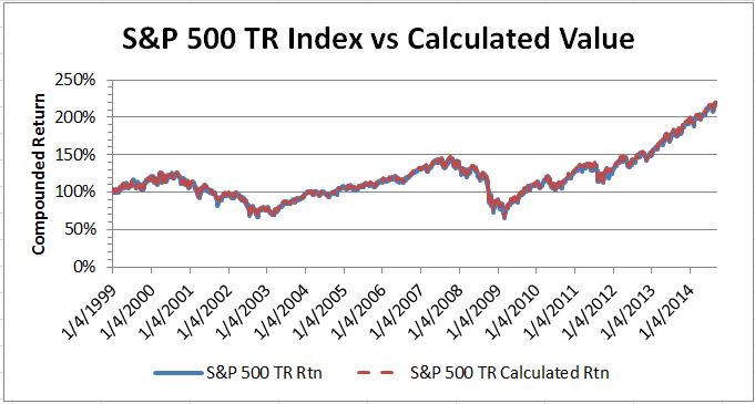
I think I found out how to do this accurately. The key was to compare the Total Return (TR) Index versus the calculation. Deriving the more widely used Price Index turns out to be a lot more complicated due to the ways in which S&P accounts for corporate actions.
In the Series Tool…
Universe: S&P 500 Index
Rule 1: setVar(@Num, UnivSum(“SharesCur(1) != NA AND Close(0) != NA AND Close(1) != NA”, “(isNA(FloatPct/100,1)SharesCur(1))(Close(0)-Close(1))”))
Rule 2: SetVar(@Denom, UnivSum(“SharesCur(1) != NA AND Close(0) != NA AND Close(1) != NA”, “isNA(FloatPct/100,1)*SharesCur(1)*Close(1)”))
Rule 3: SetVar(@Idx, @Num/@Denom)
The result is the percent return. Taking the compounded product of the percent returns (i.e., Sum[Product(1+r[t])] ) measured against the S&P 500 Total Return Index produced almost an exact match which shows a correlation coefficient of .999748 and beta coefficient of .999912. Graphically, this looks like:
Why did you use floating shares outstanding in your calculation instead of total shares outstanding? Not sure I understand the logic there.
To convert the percent return series you got from the series tool into an indexed $ series (the graph you posted), I think you had to finish the last step in Excel. Is that right? Is it possible to do it all within P123 so that the custom index can be used in sims?
I used floating shares because that is how the S&P 500 is calculated, according to the above documentation.
And you are correct that I finished in Excel. Using the cumulative feature in the Series Tool, it should be possible to do this in P123 if you convert the percent returns into log returns. You can add log returns, but not percent returns. To convert the cumulative log returns back into percent, you take it to the power of e (natural exponent)…
I think you lost me at the end. How do you convert the cumulative log return index into a cumulative total return index within the series tool? The last line in my rules tab is: LN(UnivAvg(“TRUE”,“close(0)/close(1)”)). Then I applied “Transform: cumulative” on the charts tab and I believe that created the equal weighted cumulative log return index on the chart tab. However, there’s no option after that within the series tool to do further math on the series values. Am I missing something?
The only option I see is that within a sim, you could do e^(Close(0,GetSeries"$CustomSeries")) to convert the cumulative log return index value to the the cumulative total return index value. However, you wouldn’t be able to use the SMA function (or most TA indicators) since averages of log returns aren’t the same as averages of simple returns, right?
So, I think your presumption that your formula will create an equal $ weighted is correct.
You are also correct that I meant for the exponent to be applied outside the Series Tool. While I can’t think of anyway to get a cumuluative percent return in the Series Tool given current syntax, you could certainly use something like 2.78^GetSeries(“”) in a Port/Sim.
So while the MA of a cumulative percent vs cumulative log return graph I don’t think are numerically equivalent, I believe that you circumvent this issue through algebraic manipulation such as:
Yes, I do understand why the first inequality is true, and I understand why the second equation is true. However, I tried SMA(20,0,2.718^GetSeries(“”)) and I got an invalid series error message. Seems like the syntax doesn’t work. Let me know if you or anyone sees a way. If not, I’ll create a feature request for a Transform:Multiplicative option in the series tool so that we can create cumulative total return indexes.